
ClickHouse SQL Experiment: Building a Pseudo Bloom Filter
Rethinking data filtering with a simple SQL experiment and surprising results


Introduction
This experiment allows us to explore ClickHouse’s capabilities in greater depth and look at SQL queries from a different angle. Query optimization and the search for unexpected solutions make working with ClickHouse especially interesting. The goal of this article is to inspire you to pursue new experiments and unconventional ideas!
Part 1: Intro to ClickHouse and the key features I will use in this experiment
ClickHouse is a high-performance, column-oriented DBMS designed for OLAP workloads. It can execute aggregated queries in milliseconds or seconds. However, this architecture also has limitations, especially when working with large joins in distributed environments. That’s why query optimization sometimes comes down to minimizing JOIN usage.
ClickHouse supports many useful features that will be important for this experiment:
Common Table / Scalar Expressions (CTE/CSE):
Allow you to replace repeated code defined inWITHclauses or declare aliases for arbitrary scalar expressions that can be reused throughout the query. More detailsHash functions:
ClickHouse provides multiple built-in hash functions, such as:cityHash64, murmurHash2_64. More detailsBitmap functions:
Used for working with Roaring bitmaps. I will need thebitmapContainsfunction. More detailsAggregate functions:
ClickHouse supports a wide range of aggregate functions. I will usegroupBitmapState. More details
Part 2: Intro to Bloom Filters
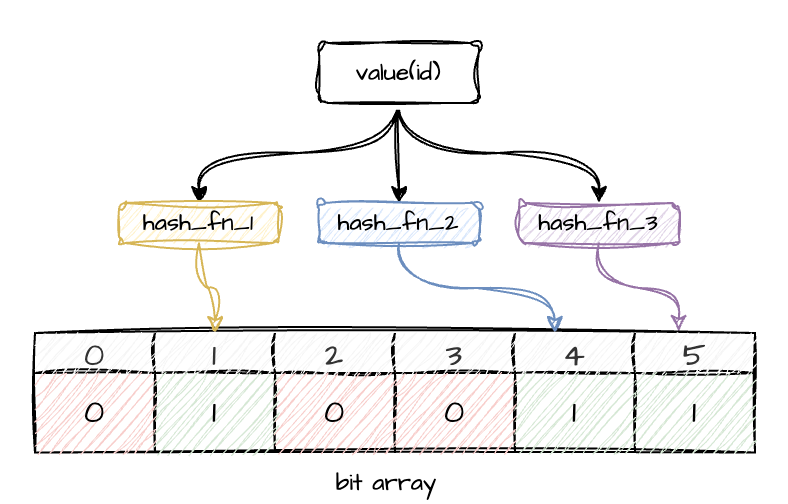
A Bloom filter is a probabilistic data structure that makes it possible to check whether an element is not present in a dataset. If the Bloom filter returns 0 for an element, it is definitely absent. If it returns 1, the element may be present — or this may be the result of a hash collision. The main goal is to reduce the probability of false positives and minimize memory lookups during checks.
Bloom filters are widely used in many areas: spam filtering, databases, recommendation systems, duplicate detection.
Graphically, it looks something like this:
Part 3: Preparing ClickHouse tables
You may already have a ClickHouse instance available for experiments, or you might be using ClickHouse Cloud. If not, you can quickly spin up a local instance using Docker.
docker run -d \
  --name some-clickhouse-server \
  --ulimit nofile=262144:262144 \
  clickhouse/clickhouse-server
Then open the Exec tab in the UI and run:
clickhouse-clientI will create two simple tables for the experiment.
Locations table:
CREATE TABLE IF NOT EXISTS locations (
    location_id UInt32,
    name        String,
    type        String   -- e.g. ‘store’, ‘online-store’
)
ENGINE = MergeTree
ORDER BY location_id;
Sales table:
CREATE TABLE IF NOT EXISTS sales (
    sale_id     UInt64,
    client      String,
    location_id UInt32,
    amount      Float64,
    ts          DateTime
)
ENGINE = MergeTree
ORDER BY (client, location_id, ts);
I won’t focus on schema design or optimization — this is outside the scope of the article.
Now let’s populate both tables with random data:
200 locations
~70% of them marked as
store100M sales records
10% of sales belonging to a controlled client
‘xxx’random
location_idvalues
INSERT INTO locations
SELECT
    number AS location_id,
    concat('Location_', toString(number)) AS name,
    if(rand() % 10 < 7, 'store', 'online-store') AS type
FROM numbers(200);
INSERT INTO sales
SELECT
number AS sale_id,
if(rand() % 10 = 0, 'xxx', concat('client_', toString(rand() % 10000))) AS client,
rand() % 200 AS location_id,
rand() % 10000 / 100 AS amount,
now() - rand() % 100000 AS ts
FROM numbers(100_000_000);With this data in place, we can move on to the experiment.
Part 4: Implementing a Pseudo Bloom Filter in ClickHouse
Here is where the fun begins.
I imitate Bloom-filter-like behavior using SQL only, combining hash projections with Roaring Bitmap functions. This is not a real Bloom filter, but a lightweight, experimental prefilter.
Concept Overview
To approximate Bloom-filter semantics, I use the following components:
groupBitmapState— stores a compressed set of integersbitmapContains— checks whether a given integer appears in that setcityHash64/murmurHash2_64— act as independent hash functions to generate projections% N— reduces hash values into a small space
How This Compares to a Classical Bloom Filter
A traditional Bloom filter consists of:
a fixed-size bit array of length M, and
k independent hash functions.
To insert a value x:
set bits at positions h1(x), h2(x), …, hk(x).
To test a value x:
check that all corresponding bits are set to 1.
If any bit is 0 → the element is definitely not present.
If all bits are 1 → the element may be present (false positives possible).
In this experiment, instead of manipulating bits directly, I store hashed projections inside Roaring Bitmaps and test for membership via bitmapContains. The mechanics are different, but the behavioral pattern is similar enough for exploration.
Step-by-Step SQL Breakdown
1. Compute hash projections
WITH
    cityHash64(location_id) % 512 AS bloom_h1,
    murmurHash2_64(location_id) % 512 AS bloom_h2,
Here I generate two independent hash values per location_id, reducing them into a 512-slot integer space. The smaller the space, the more collisions — which is desirable for a probabilistic filter experiment.
2. Build bitmap “filters”
(
    SELECT
        groupBitmapState(bloom_h1),
        groupBitmapState(bloom_h2)
    FROM locations
    WHERE type = 'store'
) AS bloom_filter
This creates two Roaring Bitmaps containing the hash projections of all store locations.
3. Apply the pseudo Bloom filter to the fact table
After building the two bitmap “filters” from the locations table, I can immediately apply them to the sales fact table. Both bitmap checks must return 1 for a row to be considered a potential match.
SELECT count(1)
FROM sales
WHERE client = 'xxx'
  AND bitmapContains(bloom_filter.1, bloom_h1)
  AND bitmapContains(bloom_filter.2, bloom_h2)
Here:
bitmapContains(bloom_filter.1, bloom_h1)checks whether the first hash projection oflocation_idappears in the bitmap built from allstorelocations.bitmapContains(bloom_filter.2, bloom_h2)performs the same check for the second hash projection.
Only rows where both projections match pass the filter. This effectively acts as a probabilistic prefilter (in fact: any false positives arise purely from hash collisions): if either hashed value is missing from its bitmap, the row is definitely not associated with a store location.
Despite using Roaring Bitmaps rather than a real Bloom filter, the behavior is conceptually similar — the filter quickly excludes values that cannot belong to the target set, without performing a traditional JOIN.
Part 5: Performance Measurements
To understand how the pseudo Bloom filter behaves compared to a traditional filtering approach, I measured the execution time, memory usage, and CPU characteristics of three identical runs for each method. All queries were executed with:
SETTINGS enable_filesystem_cache = 0I compare two approaches:
A regular
JOINbetweensalesandlocationsThe pseudo Bloom filter without
JOIN
1. Baseline: Classic JOIN
SELECT count(1)
FROM sales s
JOIN locations l ON s.location_id = l.location_id
WHERE s.client = 'xxx'
  AND l.type = 'store'
SETTINGS enable_filesystem_cache = 0;
2. Pseudo Bloom Filter Query
WITH
    cityHash64(location_id) % 512 AS bloom_h1,
    murmurHash2_64(location_id) % 512 AS bloom_h2,
    (
        SELECT
            groupBitmapState(bloom_h1),
            groupBitmapState(bloom_h2)
        FROM locations
        WHERE type = 'store'
    ) AS bloom_filter
SELECT count(1)
FROM sales
WHERE client = 'xxx'
  AND bitmapContains(bloom_filter.1, bloom_h1)
  AND bitmapContains(bloom_filter.2, bloom_h2)
SETTINGS enable_filesystem_cache = 0;
Collected Metrics
Metrics were taken from system.query_log after each execution.
Below is the summary of three runs for each method.
JOIN Results
Run | Duration (ms) | Memory (MiB) | Read Bytes | userCPU | systemCPU
1   | 50	    | 40.90	   |150,427,203 | 212,498 | 71,190
2   | 46	    | 46.56	   |150,427,203	| 209,157 | 58,608
3   | 47	    | 43.49	   |150,427,203	| 216,383 | 76,952
Pseudo Bloom Filter Results
Run | Duration (ms) | Memory (MiB) | Read Bytes | userCPU | systemCPU
1   | 44	    | 6.09	   |103,924,368 | 261,382 | 3,440
2   | 57	    | 6.09	   |103,924,368	| 341,508 | 13,538
3   | 49	    | 6.09	   |103,924,368	| 269,981 | 19,720
Interpretation of the Results
JOIN is predictable, stable, and faster — expected, since ClickHouse is heavily optimized for such patterns.
The pseudo Bloom approach uses significantly less memory — around 6 MiB vs ~45 MiB, likely due to bitmaps store at most a few hundred integers, while JOIN builds a hash table. It also reads less data, which is expected.
At the same time, the pseudo Bloom filter puts more load on user CPU (hashing 100M rows is expensive), but noticeably reduces system CPU usage.
Production Note
Although this experiment demonstrates an interesting behavior, the pseudo Bloom filter is not intended as a production technique.
For real workloads, ClickHouse provides highly optimized mechanisms such as:
dictionaries
efficient
INsubqueriesJOIN optimizations
projections
For example:
SELECT count(1)
FROM sales AS s
WHERE s.client = 'xxx'
  AND s.location_id IN (
      SELECT location_id
      FROM locations
      WHERE type = 'store'
  );
These approaches are more reliable and predictable for production environments.
Conclusions
This isn’t something you would use in production.
It’s not a way to speed up queries — it’s simply an experiment in the spirit of “what happens if I try this?”. And in that sense, the experiment was successful.

Thank you for sharing, very interesting 👏