8 Advanced Polars Functions That Save Hours in Data Work

Boost speed with the Lazy API and write faster Polars code using built-in tools

Image created with AI by Dall-E

Originally published on Medium → read here

When I first started using Polars, the API was still young (py-0.16.*) and a lot has changed since then. Over the years, Polars has matured into one of the fastest data processing libraries available.

Following its development through release notes and real-world workloads has taught me one thing: you can’t get the full performance of Polars just by writing “Pandas-style code with different syntax”. The real speed comes from understanding its built-in tools and using them correctly.

That’s why I put together this list. These are not the most obvious or commonly repeated functions — they’re the practical tools that consistently save time, reduce memory usage, and make pipelines cleaner in real production environments.

For me, Polars became not just a Pandas alternative, but a primary tool for data processing and analytics. Learning the polars-API pays off a lot in real projects, letting you solve many problems quickly with powerful features out of the box.

Of course, this list of 8 functions isn’t exhaustive. I intentionally excluded widely used methods you’ve probably applied many times — the whole point here is to talk about something more practical and less obvious.

Below are 8 Polars functions that have helped me in production:

• value_counts

• rolling

• with_row_index

• lazy

• pipe

• map_elements

• iter_slices

• vstack

The full code for exploration and execution is available here

Data Preparation and DataFrame Creation

To simplify things, I will reuse the DataFrame creation code from one of my other articles. We have the following data:

• online_store — the store identifier

• product_id — product ID

• quantity — number of purchased or viewed items

• action_type — action type (view or purchase)

• action_dt — timestamp of the action

Requirements:

polars==1.33.0
numpy==2.3.3
graphviz

Code snippet:

from datetime import datetime, timedelta
from random import choice, gauss, randrange, seed

import polars as pl
import numpy as np


# results are replicable
seed(42)


base_time: datetime = datetime(2024, 8, 9, 0, 0, 0, 0)
num_records: int = 1_000_000

user_actions_data: list[dict] = [
    {
        "online_store": choice(["Shop1", "Shop2", "Shop3"]),
        "product_id": choice(["0001", "0002", "0003"]),
        "quantity": choice([1.0, 2.0, 3.0]),
        "action_typ": ("purchase" if gauss() > 0.6 else "view"),
        "action_dt": base_time - timedelta(minutes=randrange(num_records)),
    }
    for x in range(num_records)
]
user_actions_df: pl.DataFrame = pl.DataFrame(user_actions_data)

1. Using value_counts

This is my go-to tool for catching anomalies when the data is supposed to follow categories or types. Once, I had to debug metric discrepancies between two datasets from different parts of a workflow. Based on intuition, I suspected a mismatch between categories. Luckily, there weren’t many categories, and using value_counts() directly in the CLI helped me spot those mismatches instantly.

Example:

(
  user_actions_df
    .select(pl.col('online_store'))
    .to_series()
    .value_counts()
)

online_store count
“Shop1” 332835
“Shop2” 333569
“Shop3” 333596

It’s also great for exploratory analysis and is a very quick way to check distribution across groups:

(
  user_actions_df
    .select(pl.col('online_store'))
    .to_series()
    .value_counts(sort=True, normalize=True)
)

online_store proportion
“Shop3” 0.333596
“Shop2” 0.333569
“Shop1” 0.332835

Useful documentation (official Polars references for deeper exploration)

polars.Series.value_counts | polars.Expr.value_counts

2. Using rolling

A powerful tool for time-series or ordered sequences where you need smoothing windows, fill missing values with rolling averages, and so on. The function is easy to use, but it’s important to remember that index_column only works with Date/Datetime or integer types.

If you want to use rolling based on an index but you don’t have one, combine rolling() with with_row_index().

Example:

user_actions_df
  .sort('action_dt')
  .rolling(index_column='action_dt', period='1h').agg(
      sum_quantity = pl.sum('quantity'),
      agg_quantity = pl.col('quantity'),
      agg_action_dt = pl.col('action_dt'),
).head()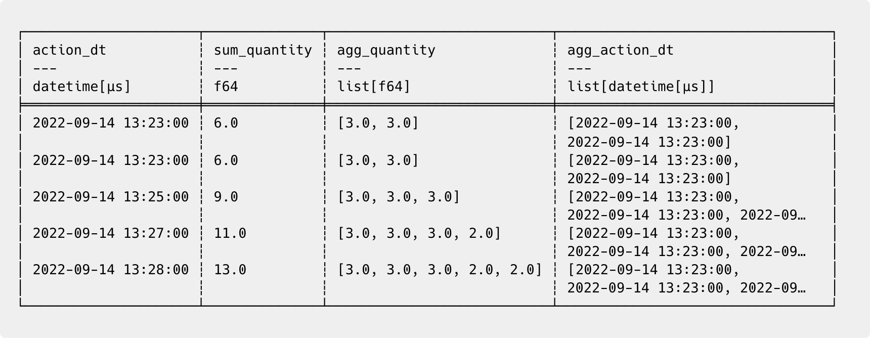

If you need calculations per group rather than by sequential order, use .over() instead.

Useful documentation (official Polars references for deeper exploration)

polars.DataFrame.rolling | polars.LazyFrame.rolling | polars.Expr.rolling

3. Using with_row_index

A Polars DataFrame is not the same as a Pandas DataFrame, and if you need an index, the simplest way is to generate one with with_row_index(). I needed it once to restore the original ordering of modified rows — rare case, but useful to know.

Example:

user_actions_df.with_row_index('id').head()

id online_store product_id quantity action_type action_dt
0 “Shop3” “0001” 1.0 “view” 2024-04-29 09:24:00
1 “Shop3” “0001” 3.0 “view” 2023-02-16 15:54:00
2 “Shop3” “0001” 3.0 “view” 2024-03-02 19:02:00
3 “Shop1” “0003” 3.0 “view” 2024-07-20 16:16:00
4 “Shop3” “0001” 3.0 “view” 2024-03-01 11:32:00

Useful documentation (official Polars references for deeper exploration)

polars.DataFrame.with_row_index | polars.LazyFrame.with_row_index

4. Using lazy

The Lazy API is a mode where Polars doesn’t execute operations immediately. Instead, it builds a query plan that will be optimized and executed only after calling .collect().

Lazy mode works not only for in-memory DataFrames, but also for external sources like scan_csv, scan_parquet, scan_delta, scan_iceberg, and others. In many cases, this optimization provides a huge boost in performance and reduces memory usage. For example, projection pushdown and predicate pushdown allow reading only required columns and filtering at the source level.

Example:

lf = (
    user_actions_df
    .lazy()
    .with_columns(quantity = pl.col('quantity')**2)
    .filter(pl.col('action_type') == 'purchase')
    .select('online_store', 'action_type', 'quantity')
    .head()
)

lf.show_graph(optimized=False)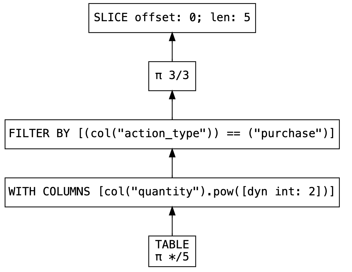

As we can see in the initial non-optimized plan (optimized=False), Polars simply repeats our instructions step by step:

• Reads the table

• Squares the quantity column

• Filters only purchases (action_type = “purchase”)

• Keeps only the necessary columns

• Takes the first 5 rows

However, because our DataFrame is lazy, none of this has been executed yet. This gives Polars the opportunity to optimize the query before execution. Let’s take a look at the optimized plan, which will actually be executed when we call collect():

• Reads only the required columns from the table

• Filters only purchases (action_type = “purchase”)

• Takes the first 5 rows

• Squares the quantity column

lf.show_graph()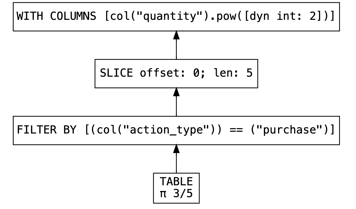

lf.collect()

online_store action_type quantity
“Shop2” “purchase” 1.0
“Shop1” “purchase” 4.0
“Shop2” “purchase” 9.0
“Shop1” “purchase” 9.0
“Shop2” “purchase” 4.0

Lazy mode in Polars doesn’t just delay execution, it restructures the query to process less data and do it as efficiently as possible.

Useful documentation (official Polars references for deeper exploration)

Lazy — Polars user guide

5. Using pipe

At first glance, pipe() may look like a tool just for organizing code, but that’s not the whole story. I recommend using pipe() particularly with LazyFrame then you get all the benefits of optimization and parallel execution.

It’s probably my favorite function for writing clean transformation pipelines:

def step1(frame: pl.LazyFrame) -> pl.LazyFrame:
    return frame.filter(pl.col('online_store') == 'Shop1')

def step2(frame: pl.LazyFrame) -> pl.LazyFrame:
    return frame.with_columns(sum_quantity=pl.col('quantity').sum())

def step3(frame: pl.LazyFrame) -> pl.LazyFrame:
    return frame.head()

(
    user_actions_df
    .lazy()
    .pipe(step1)
    .pipe(step2)
    .pipe(step3)
    .collect()
)

online_store product_id quantity action_type action_dt sum_quantity
“Shop1” “0003” 3.0 “view” 2024-07-20 16:16:00 664965.0
“Shop1” “0001” 3.0 “view” 2024-03-05 05:08:00 664965.0
“Shop1” “0002” 2.0 “view” 2023-02-24 15:01:00 664965.0
“Shop1” “0001” 3.0 “view” 2024-06-11 21:33:00 664965.0
“Shop1” “0001” 2.0 “purchase” 2024-01-19 14:04:00 664965.0

I wrote an article on how to structure code with pipe():

Improving Code Quality During Data Transformation with Polars

Useful documentation (official Polars references for deeper exploration)

polars.DataFrame.pipe | polars.LazyFrame.pipe | polars.Expr.pipe

6. Using map_elements

Polars supports several UDF types, and map_elements is one of them. It’s great when you need to extract complex business logic into a separate function. Libraries like NumPy and SciPy also provide ready ufuncs, which you can use inside UDFs.

Just remember that UDFs are not as optimal as native Polars expressions — so use them wisely.

Example:

user_actions_df.select(pl.col('quantity').map_elements(np.log)).head()

For a detailed exploration of all UDF options, I wrote this article:

Understanding Polars UDF Capabilities

Useful documentation (official Polars references for deeper exploration)

polars.Series.map_elements | polars.Expr.map_elements

7. Using iter_slices

A simple but extremely useful function when you need to control batching and writing to a database or file, or sending data somewhere in chunks. Some people generate indexes to iterate, but it’s much better to use iter_slices() instead.

for idx, frame in enumerate(user_actions_df.iter_slices(n_rows=100_000)):
    print(f"{type(frame).__name__}[{idx}]: {len(frame)}")

DataFrame[0]: 100000
DataFrame[1]: 100000
DataFrame[2]: 100000
DataFrame[3]: 100000
DataFrame[4]: 100000
DataFrame[5]: 100000
DataFrame[6]: 100000
DataFrame[7]: 100000
DataFrame[8]: 100000
DataFrame[9]: 100000

If you need slicing by groups, use .group_by() instead — the returned object GroupBy is iterable.

Useful documentation (official Polars references for deeper exploration)

polars.DataFrame.iter_slices

8. Using vstack

If you have multiple DataFrames with identical schemas or you’re processing history iteratively and want to save everything together — this method is perfect. Don’t forget to call rechunk() at the end.

If you plan to perform transformations after adding data, consider using .extend():

• vstack(): fast concatenation, but creates many chunks → requires rechunk() later.

• extend(): a bit more expensive per insert, but the intermediate dataframe stays fast to operate on.

If you need to concatenate DataFrames using different strategies, use concat()

Example:

buffer: pl.DataFrame = pl.DataFrame()

for name, chunk in user_actions_df.group_by('online_store'):
    buffer.vstack(chunk,in_place=True)
    print(f">>> {name[0]} <<<")
    chunk.glimpse(max_items_per_column=1)

print(f">>> Result <<<")
buffer.glimpse(max_items_per_column=3)

# n_chunks - get number of chunks used by the ChunkedArrays of this DataFrame: 
print(f"Before rechunk(): {buffer.n_chunks(strategy='all')}")
buffer = buffer.rechunk()
print(f"After rechunk(): {buffer.n_chunks(strategy='all')}")

>>> Shop1 <<<
Rows: 332835
Columns: 5
$ online_store          <str> ‘Shop1’
$ product_id            <str> ‘0003’
$ quantity              <f64> 3.0
$ action_type           <str> ‘view’
$ action_dt    <datetime[μs]> 2024-07-20 16:16:00

>>> Shop2 <<<
Rows: 333569
Columns: 5
$ online_store          <str> ‘Shop2’
$ product_id            <str> ‘0003’
$ quantity              <f64> 2.0
$ action_type           <str> ‘view’
$ action_dt    <datetime[μs]> 2022-12-28 14:11:00

>>> Shop3 <<<
Rows: 333596
Columns: 5
$ online_store          <str> ‘Shop3’
$ product_id            <str> ‘0001’
$ quantity              <f64> 1.0
$ action_type           <str> ‘view’
$ action_dt    <datetime[μs]> 2024-04-29 09:24:00

>>> Result <<<
Rows: 1000000
Columns: 5
$ online_store          <str> ‘Shop1’, ‘Shop1’, ‘Shop1’
$ product_id            <str> ‘0003’, ‘0001’, ‘0002’
$ quantity              <f64> 3.0, 3.0, 2.0
$ action_type           <str> ‘view’, ‘view’, ‘view’
$ action_dt    <datetime[μs]> 2024-07-20 16:16:00, 2024-03-05 05:08:00, 2023-02-24 15:01:00

Before rechunk(): [3, 3, 3, 3, 3]
After rechunk(): [1, 1, 1, 1, 1]

Useful documentation (official Polars references for deeper exploration)

polars.DataFrame.vstack | polars.DataFrame.extend | polars.concat

Summary

Polars come with a lot of powerful features out of the box. Knowing the right ones can dramatically improve both performance and code quality in production pipelines.

---